The software accepts data in comma-separate values (csv) format. Columns should represent features/variables and rows should represent conditions or samples, see Table 1. Data should have a column header indicating feature names (shaded blue in Table 1) and row header indicating condition names (shaded grey in Table 1).
The data in ShapoGraphy should be scaled between 0 and 1.0. Dimensional data (i.e. length, width, ..) should be scaled between 0.1 and 1.0 to avoid diminishing of the smallest object. Dimensional data should be scaled in a way that their ratios (w/l) before and after normalization is equal. For example, if the largest object length is l1=100 and width w1=50, then l1'=1 and w1=.5.
You can also normalize your data in our app using the Normalise data sub-menu on the right. There, you can select the dimensional variables if applicable.
Table 1: Example on the format of the data that can be uploaded to ShapoGraphy
Condition
Cell length
Cell width
Number of nuclei
Nucleus length
Nucleus width
Control
0.5
0.4
2
0.4
0.3
Condition 1
0.9
0.5
4
0.5
0.35
Condition 2
0.6
0.45
5
0.3
0.3
Condition 3
0.8
0.5
7
0.5
0.45
Condition 4
0.4
0.2
6
0.2
0.2
To plot your data using ShapoGraphy you need to first upload data. Currently ShapoGraphy support comma separated files (i.e. csv files, see File format). Add objects to represent map your data to using the shapes on the left menu (e.g. an ellipse for a cell or tumour, a square for a well, or draw your own shape).
gesture
Draw square
Draw circle
Draw hexagon
Draw triangle
Draw rounded rectangle
Draw semi-circle
Draw custom
The added objects will be displayed on right menu (see Objects menu) where their names, locations relative to each other and initial size can be customized in the Global features menu.
The color of an object can be static (fixed for all samples) or dynamic (vary across samples depending on a selected variable value). If you wish to use a static color, you can adjust it from the color picker in the left menu where you can also adjust the object stroke color.
Features
Several features can be mapped to each object as detailed below. The user can show/hide a certain visual element by clicking on the eye icon.
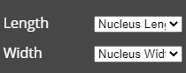
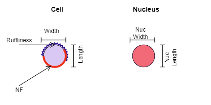
Object dimensions:
Length: object length or height
Width: object width. If you only have one dimensional variable (e.g. area, or radius) then select the same feature for length and width.
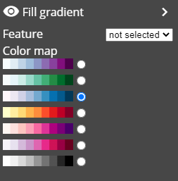
Fill gradient: this element assigns a color for each object instance based on the value of the selected variable and the chosen gradient as in a heat map
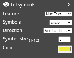
Fill Symbols: this element fills the object with symbols propotional to the selected variable value.
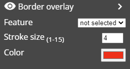
Border overlay: this element plots part of object border as a thick line. The extent of the thick line is propotional to the selected feature value. The color of the thick line can be specified. This element can be used to represent the extent of cell crowding or adhesion
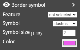
Border overlay symbols: this element plots symbols on the border of the object propotional to the selected variable value. You can sepcify the symbole (e.g. dashes, star or dots).
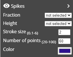
Spikes: this element can represent irregularity in the object shape or spread of the object (e.g. spread of tumour). It extends around the object border proportional to the selected variable value.
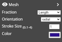
Mesh: this element can represent selected feature values as the density of mesh. The user have a choice of vertical, horizontal, radial, grid, or random grid mesh. For example the density of horizontal lines can represent fiber density
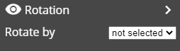
Rotation: the object will be rotated depending on the variable value.
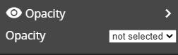
Opacity: the transperency of the object will be depending on the variable value.
ShapoGraphy requirements
For best experience, run ShapoGraphy using Google Chrome.
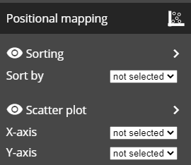
Positional mapping
This section allows you to sort glyphs based on a certain variable, or arrange them in a scatter plot by choosing X and Y variabless
Sorting
You can select variables To sort plotted glyph sets based on the value of a designated variable.
Scatter plot
To arrange plotted glyph sets in a scatter plot, you can select variables to position them on the x- and y-axis. This help sorting the glyphs or further group them and effectively add additional dimensions.
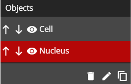
Objects menu
The object menu contains a list of the objects you have created
From here, you can manipulate your objects as follows:
Change the order of the objects using the north south icons
Change the objects' visibility using the remove_red_eye icon
Rename the objects using the edit icon at the bottom of objects list
Replicate the objects using the content_copy icon at the bottom of objects
Delete the objects using the delete icon at the bottom of objects
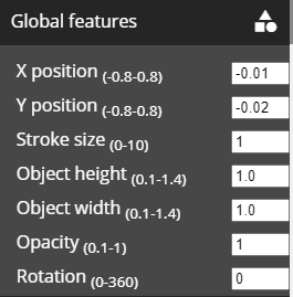
Global features
The global features menu contain features that will be equally applied to the object across all data points (rows in the data file)
Available global features include:
Changing the position of the object on the X-axis
Changing the position of the object on the Y-axis
Changing the stroke size of the object
Changing the object's height
Changing the object's width
Changing the object's opacity
The angle of the object
Object Positions relative to the center of the cluster can also be specified interactively by dragging and dropping the object
Loading and saving
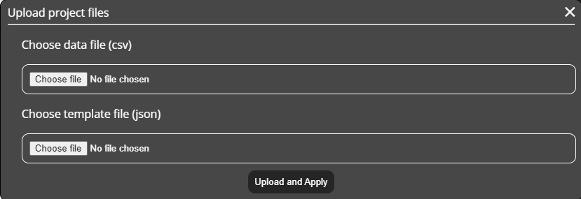
An additional option to load your data to our page is selecting the load project option from the file menu
this will open a window where you can select your data.csv file and any previous template.json file you worked on earlier
this will load the dataset and apply the template to it at the same time
Please notice that the template.json file must contain values with similar feature names. If you load a dataset with different feature names then you need to map your features to the object elements again.
Additional saving options include:
Save template: to save the design and data mapping as a json file select File -> save template.
Save Svg: to save the plot as a SVG file, select File -> save SVG.
Save PNG: to save the plot as a PNG file, select File -> save PNG.
Figure legend
You can view the legend specifying the feature mapping to different glyph objects by clicking the legend button in the top menu
You can also save this legend as a SVG file or a PNG image by selecting the save legend option from the file menu
Additional views
Addition views in ShapoGraphy include:
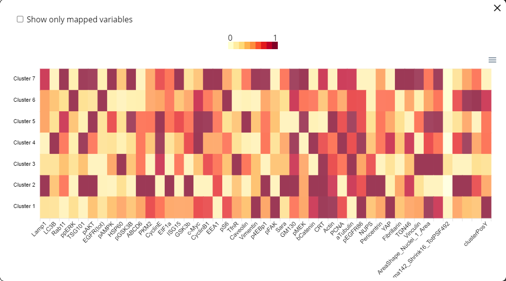
Heat map
Accessed by clicking the heatmap button in the top menu.
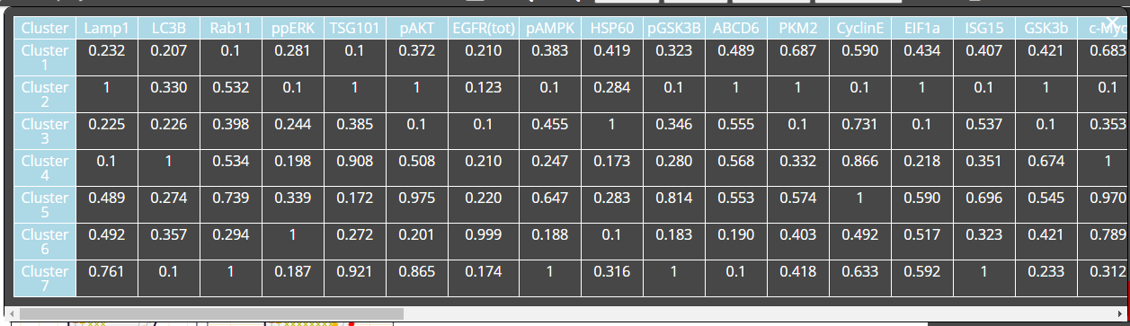
Data table
Shows the dataset values in a table for ease of access Accessed by clicking the Table icon option in the top menu*.
*The dataset option becomes visible only after loading a data file
Zooming
The user can zoom in or zoom out on any point on the canvas
This is done by clicking the Zoom in icon and then moving the mouse pointer to the desired point and scrolling the mouse wheel to zoom in or out
To cancel the zooming operation, simply click the Zoom out icon which will revert the canvas to it's original state
Using templates
Shapography introduces pre-designed templates which the user can use with their own datasets
On the homepage, you can find them in the templates section, click on the template that you like to see and it will be rendered on the canvas before you
At that point, the template will be using a mock dataset for the sake of demonstration, you can load one of our datasets to apply the template to them, or simply use your own
At the moment most templates have their own tutorials which would be indicated at the top of the rendered canvas, you can also access them through the 'Help' tab in the navbar
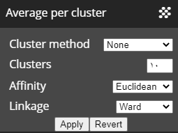
Clustering
When a large dataset that contains a minimum of 50 rows or more, the user can use the average per cluster feature
This feature will allow the user to cluster the data using the selected method and show clusters based on the average of the generated clusters values